정규 분포
개요
- 고교 과정의 통계에서는 정규분포의 기본적인 성질과 정규분포표 읽는 방법을 배움.
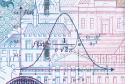
- 평균이 <math>\mu</math>, 표준편차가 <math>\sigma</math>인 정규분포의 <math>N(\mu,\sigma^2)</math>의 확률밀도함수, 즉 가우시안은 다음과 같음이 알려져 있음.:<math>\frac{1}{\sigma\sqrt{2\pi}}\exp\left(-\frac{(x-\mu)^2}{2\sigma^2}\right)</math>
- 아래에서는 이 확률밀도함수가 어떻게 해서 얻어지는가를 보임.(기본적으로는 가우스의 증명)
- 가우시안의 형태를 얻는 또다른 방법으로 드무아브르-라플라스 중심극한정리 를 참조.
'오차의 법칙'을 통한 가우시안의 유도
- 오차 = 관측하려는 실제값 - 관측에서 얻어지는 값
- 오차의 분포를 기술하는 확률밀도함수 <math>\Phi</math>는 다음과 같은 성질을 만족시켜야 함. 1) <math>\Phi(x)=\Phi(-x)</math> 2)작은 오차가 큰 오차보다 더 나타날 확률이 커야한다. 그리고 매우 큰 오차는 나타날 확률이 매우 작아야 한다. 3) <math>\int_{-\infty}^{\infty} \Phi(x)\,dx=1</math> 4) 관측하려는 실제값이 <math>\mu</math> 이고, n 번의 관측을 통해 <math>x_ 1, x_ 2, \cdots, x_n</math> 을 얻을 확률 <math>\Phi(\mu-x_ 1)\Phi(\mu-x_ 2)\cdots\Phi(\mu-x_n)</math>의 최대값은 <math>\mu=\frac{x_ 1+x_ 2+ \cdots+ x_n}{n}</math>에서 얻어진다.
- 4번 조건을 가우스의 산술평균의 법칙이라 부르며, 관측에 있어 실제값이 될 개연성이 가장 높은 값은 관측된 값들의 산술평균이라는 가정을 하는 것임.
- 정리 (가우스)
이 조건들을 만족시키는 확률밀도함수는 <math>\Phi(x)=\frac{h}{\sqrt{\pi}}e^{-h^2x^2}</math> 형태로 주어진다. 여기서 <math>h</math>는 확률의 정확도와 관련된 값임. (실제로는 표준편차와 연관되는 값)
- 증명
<math>n=3</math>인 경우에 4번 조건을 만족시키는 함수를 찾아보자.
<math>\Phi(x-x_ 1)\Phi(x-x_ 2)\Phi(x-x_ 3)</math>의 최대값은 <math>x=\frac{x_ 1+x_ 2+ x_ 3}{3}</math> 에서 얻어진다.
따라서 <math>\ln \Phi(x-x_ 1)\Phi(x-x_ 2)\Phi(x-x_ 3)</math> 의 최대값도 <math>x=\frac{x_ 1+x_ 2+ x_ 3}{3}</math> 에서 얻어진다.
미분적분학의 결과에 의해, <math>x=\frac{x_ 1+x_ 2+ x_ 3}{3}</math> 이면, <math>\frac{\Phi'(x-x_ 1)}{\Phi(x-x_ 1)}+\frac{\Phi'(x-x_ 2)}{\Phi(x-x_ 2)}+\frac{\Phi'(x-x_ 3)}{\Phi(x-x_ 3)}=0</math> 이어야 한다.
<math>F(x)=\frac{\Phi'(x)}{\Phi(x)}</math> 으로 두자.
<math>x+y+z=0</math> 이면, <math>F(x)+F(y)+F(z)=0</math> 이어야 한다.
1번 조건에 의해, <math>F</math> 는 기함수이다.
따라서 모든 <math>x,y</math> 에 의해서, <math>F(x+y)=F(x)+F(y)</math> 가 성립한다. 그러므로 <math>F(x)=Ax</math> 형태로 쓸수 있다.
이제 적당한 상수 <math>B, h</math> 에 의해 <math>\Phi(x)=Be^{-h^2x^2}</math> 꼴로 쓸 수 있다.
모든 <math>n</math>에 대하여 4번조건이 만족됨은 쉽게 확인할 수 있다. (증명끝)
역사
- 중심극한정리는 여러 과정을 거쳐 발전
- 이항분포의 중심극한 정리
- 라플라스의 19세기 초기 버전
확률변수 X가 이항분포 B(n,p)를 따를 때, n이 충분히 크면 X의 분포는 근사적으로 정규분포 N(np,npq)를 따른다
- 드무아브르가 18세기에 발견한 것은 이항분포에서 확률이 1/2인 경우
- 드무아브르-라플라스 중심극한정리 의 유도는 해당 항목을 참조.
- 수학사 연표
재미있는 사실
- 정규분포와 중심극한정리에 대한 이해는 교양인이 알아야 할 수학 주제의 하나
- Galton's quincunx
- 정규분포의 밀도함수 형태를 물리적으로 얻을 수 있는 장치.
- http://ptrow.com/articles/Galton_June_07.htm
- 예전 독일 마르크화에는 가우스의 발견을 기려 정규분포곡선이 새겨짐

관련된 항목들
계산 리소스
- 동전던지기 시뮬레이션
- 자바애플릿
관련도서
- Fischer, Hans , History of the Central Limit Theorem : From Laplace to Donsker
- The History of Statistics: The Measurement of Uncertainty before 1900
- Excursions in calculus
- 206~216p, The law of errors
사전형태의 자료
- http://ko.wikipedia.org/wiki/중심극한정리
- http://ko.wikipedia.org/wiki/정규분포
- http://en.wikipedia.org/wiki/normal_distribution
- http://en.wikipedia.org/wiki/Central_limit_theorem
- http://viswiki.com/en/central_limit_theorem
- 다음백과사전 http://enc.daum.net/dic100/search.do?q=오차의법칙
에세이
- http://math.stackexchange.com/questions/28558/what-do-pi-and-e-stand-for-in-the-normal-distribution-formula
- Pearson, Karl. "Historical note on the origin of the normal curve of errors." Biometrika (1924): 402-404. http://biomet.oxfordjournals.org/cgi/reprint/16/3-4/402.pdf
관련기사
- 과학자들의 진실게임 - 그 법칙은 내꺼야!
- 과학에서 최초의 발견자와 크레딧 논쟁 사례
- 한겨레, 2008-10-10
- [재미있는 과학이야기 통계의 기본원리 ② 가우스 분포]
- 주간한국, 2008-01-07
- 기사 검색 (키워드 수정)
블로그
- 피타고라스의 창
동영상
노트
위키데이터
- ID : Q133871
말뭉치
- Normal distribution, also called Gaussian distribution, the most common distribution function for independent, randomly generated variables.[1]
- Read More on This Topic statistics: The normal distribution The most widely used continuous probability distribution in statistics is the normal probability distribution.[1]
- normal distribution , sometimes called the bell curve, is a distribution that occurs naturally in many situations.[2]
- For example, the bell curve is seen in tests like the SAT and GRE.[2]
- A smaller standard deviation indicates that the data is tightly clustered around the mean; the normal distribution will be taller.[2]
- If the data is evenly distributed, you may come up with a bell curve.[2]
- Everything we do, or almost everything we do in inferential statistics, which is essentially making inferences based on data points, is to some degree based on the normal distribution.[3]
- And so what I want to do in this video and in this spreadsheet is to essentially give you as deep an understanding of the normal distribution as possible.[3]
- And it actually turns out, for the normal distribution, this isn't an easy thing to evaluate analytically.[3]
- and if you were to take the sum of them, as you approach an infinite number of flips, you approach the normal distribution.[3]
- You can see a normal distribution being created by random chance![4]
- From the big bell curve above we see that 0.1% are less.[4]
- Use the Standard Normal Distribution Table when you want more accurate values.[4]
- The normal distribution is the most common type of distribution assumed in technical stock market analysis and in other types of statistical analyses.[5]
- The normal distribution model is motivated by the Central Limit Theorem.[5]
- Normal distribution is sometimes confused with symmetrical distribution.[5]
- The skewness and kurtosis coefficients measure how different a given distribution is from a normal distribution.[5]
- The case where μ = 0 and σ = 1 is called the standard normal distribution.[6]
- The normal distribution is the most important probability distribution in statistics because it fits many natural phenomena.[7]
- For example, heights, blood pressure, measurement error, and IQ scores follow the normal distribution.[7]
- The normal distribution is a probability function that describes how the values of a variable are distributed.[7]
- As with any probability distribution, the parameters for the normal distribution define its shape and probabilities entirely.[7]
- If a dataset follows a normal distribution, then about 68% of the observations will fall within of the mean , which in this case is with the interval (-1,1).[8]
- Although it may appear as if a normal distribution does not include any values beyond a certain interval, the density is actually positive for all values, .[8]
- The standardized values in the second column and the corresponding normal quantile scores are very similar, indicating that the temperature data seem to fit a normal distribution.[8]
- Let us find the mean and variance of the standard normal distribution.[9]
- To find the CDF of the standard normal distribution, we need to integrate the PDF function.[9]
- Most of the continuous data values in a normal distribution tend to cluster around the mean, and the further a value is from the mean, the less likely it is to occur.[10]
- The normal distribution is often called the bell curve because the graph of its probability density looks like a bell.[10]
- The normal distribution is the most important probability distribution in statistics because many continuous data in nature and psychology displays this bell-shaped curve when compiled and graphed.[10]
- Converting the raw scores of a normal distribution to z-scores We can standardized the values (raw scores) of a normal distribution by converting them into z-scores.[10]
- The diagram above shows the bell shaped curve of a normal (Gaussian) distribution superimposed on a histogram of a sample from a normal distribution.[11]
- The tail area of the normal distribution is evaluated to 15 decimal places of accuracy using the complement of the error function (Abramowitz and Stegun, 1964; Johnson and Kotz, 1970).[11]
- This guide will show you how to calculate the probability (area under the curve) of a standard normal distribution.[12]
- It will first show you how to interpret a Standard Normal Distribution Table.[12]
- As explained above, the standard normal distribution table only provides the probability for values less than a positive z-value (i.e., z-values on the right-hand side of the mean).[12]
- We start by remembering that the standard normal distribution has a total area (probability) equal to 1 and it is also symmetrical about the mean.[12]
- The "normal distribution" is the most commonly used distribution in statistics.[13]
- To choose the best Box-Cox transformation—the one that best approximates a normal distribution - Box and Cox suggested using the maximum likelihood method.[13]
- The graph of the normal distribution depends on two factors - the mean and the standard deviation.[14]
- To find the probability associated with a normal random variable, use a graphing calculator, an online normal distribution calculator, or a normal distribution table.[14]
- In the examples below, we illustrate the use of Stat Trek's Normal Distribution Calculator, a free tool available on this site.[14]
- The normal distribution calculator solves common statistical problems, based on the normal distribution.[14]
- In a normal distribution, data is symmetrically distributed with no skew.[15]
- Example: Using the empirical rule in a normal distribution You collect SAT scores from students in a new test preparation course.[15]
- The data follows a normal distribution with a mean score (M) of 1150 and a standard deviation (SD) of 150.[15]
- A random variable with the standard Normal distribution, commonly denoted by \(Z\), has mean zero and standard deviation one.[16]
- The probabilities for any Normal distribution can be reduced to probabilities for the standard Normal distribution, using the device of standardisation.[16]
- Crowd size Suppose that crowd size at home games for a particular football club follows a Normal distribution with mean \(26\ 000\) and standard deviation 5000.[16]
- The cdf of any Normal distribution can also be found, using technology, without first standardising.[16]
- The normal distribution is also useful when sampling data out of a non-normal data set.[17]
- A truncated NORMAL distribution can be defined for a variable by setting the desired minimum and/or maximum values for the variable.[18]
- For practical purposes, minimum and maximum values that are at least 3 standard deviations away from the mean generate a complete normal distribution.[18]
- For a Normal distribution, 99.73 % of all samples, will fall within 3 Standard Deviations of the mean value.[18]
- Many other common distributions become like the normal distribution in special cases.[19]
- Look at the histograms of lifetimes given in Figure 21.3 and of resistances given in Figure 21.4 and you will see that they resemble the normal distribution.[19]
- If you were to get a large group of students to measure the diameter of a washer to the nearest 0.1 mm, then a histogram of the results would give an approximately normal distribution.[19]
- However, there is a problem with the normal distribution function in that is not easy to integrate![19]
- The normal distribution is also referred to as Gaussian or Gauss distribution.[20]
- In a normal distribution graph, the mean defines the location of the peak, and most of the data points are clustered around the mean.[20]
- A normal distribution comes with a perfectly symmetrical shape.[20]
- The middle point of a normal distribution is the point with the maximum frequency, which means that it possesses the most observations of the variable.[20]
- We will get a normal distribution if there is a true answer for the distance, but as we shoot for this distance, since, to err is human, we are likely to miss the target.[21]
- We can use the fact that the normal distribution is a probability distribution, and the total area under the curve is 1.[21]
- If you use the normal distribution, the probability comes of to be about 0.728668.[21]
- The minimum variance unbiased estimator (MVUE) is commonly used to estimate the parameters of the normal distribution.[22]
- For an example, see Fit Normal Distribution Object.[22]
- The normal distribution is the most well-known distribution and the most frequently used in statistical theory and applications.[23]
- Any articles that did not specify the type of distribution or which referred to the normal distribution were likewise excluded.[23]
- In stage 2 we eliminated a further 292 abstracts that made no mention of the type of distribution and one which referred to a normal distribution.[23]
- Before introducing the normal distribution, we first look at two important concepts: the Central limit theorem, and the concept of independence.[24]
- The Central limit theorem plays an important role in the theory of probability and in the derivation of the normal distribution.[24]
- As one sees from the above figures, the distribution from these averages quickly takes the shape of the so-called normal distribution.[24]
- You might still find yourself having to refer to tables of cumulative area under the normal distribution, instead of using the pnorm() function (for example in a test or exam).[24]
- The normal distribution is a continuous, univariate, symmetric, unbounded, unimodal and bell-shaped probability distribution.[25]
- Use this to describe a quantity that has a normal normal distribution with the given «mean» and standard deviation «stddev».[25]
- Suppose you want to fit a Normal distribution to historical data.[25]
- The normal distribution holds an honored role in probability and statistics, mostly because of the central limit theorem, one of the fundamental theorems that forms a bridge between the two subjects.[26]
- In addition, as we will see, the normal distribution has many nice mathematical properties.[26]
- In the Special Distribution Simulator, select the normal distribution and keep the default settings.[26]
- In the special distribution calculator, select the normal distribution and keep the default settings.[26]
- Indeed it is so common, that people often know it as the normal curve or normal distribution, shown in Figure \(\PageIndex{1}\).[27]
- It is also known as the Gaussian distribution after Frederic Gauss, the first person to formalize its mathematical expression.[27]
- The normal distribution model always describes a symmetric, unimodal, bell shaped curve.[27]
- Specifically, the normal distribution model can be adjusted using two parameters: mean and standard deviation.[27]
- The normal or Gaussian distribution is extremely important in statistics, in part because it shows up all the time in nature.[28]
- The standard normal is defined as a normal distribution with μ = 0 and σ = 1.[28]
- You probably have explored the normal distribution before.[28]
- Below, you can adjust the parameters of the normal distribution and compare it to the standard normal.[28]
- For normally distributed vectors, see Multivariate normal distribution .[29]
- The simplest case of a normal distribution is known as the standard normal distribution.[29]
- Authors differ on which normal distribution should be called the "standard" one.[29]
- σ Z + μ {\displaystyle X=\sigma Z+\mu } will have a normal distribution with expected value μ {\displaystyle \mu } and standard deviation σ {\displaystyle \sigma } .[29]
- The so-called "standard normal distribution" is given by taking and in a general normal distribution.[30]
- This theorem states that the mean of any set of variates with any distribution having a finite mean and variance tends to the normal distribution.[30]
소스
- ↑ 1.0 1.1 normal distribution | Definition, Examples, Graph, & Facts
- ↑ 2.0 2.1 2.2 2.3 Normal Distributions (Bell Curve): Definition, Word Problems
- ↑ 3.0 3.1 3.2 3.3 Normal distribution (Gaussian distribution) (video)
- ↑ 4.0 4.1 4.2 Normal Distribution
- ↑ 5.0 5.1 5.2 5.3 Normal Distribution
- ↑ 1.3.6.6.1. Normal Distribution
- ↑ 7.0 7.1 7.2 7.3 Normal Distribution in Statistics
- ↑ 8.0 8.1 8.2 The Normal Distribution
- ↑ 9.0 9.1 Normal random variables
- ↑ 10.0 10.1 10.2 10.3 Normal Distribution (Bell Curve)
- ↑ 11.0 11.1 Normal Distribution and Standard Normal (Gaussian)
- ↑ 12.0 12.1 12.2 12.3 How to do Normal Distributions Calculations
- ↑ 13.0 13.1 Dietary Assessment Primer
- ↑ 14.0 14.1 14.2 14.3 Normal Distribution
- ↑ 15.0 15.1 15.2 Examples, Formulas, & Uses
- ↑ 16.0 16.1 16.2 16.3 Normal distribution
- ↑ Radiology Reference Article
- ↑ 18.0 18.1 18.2 Normal Distribution
- ↑ 19.0 19.1 19.2 19.3 Normal Distribution - an overview
- ↑ 20.0 20.1 20.2 20.3 Overview, Parameters, and Properties
- ↑ 21.0 21.1 21.2 The Normal Distribution
- ↑ 22.0 22.1 Normal Distribution
- ↑ 23.0 23.1 23.2 Non-normal Distributions Commonly Used in Health, Education, and Social Sciences: A Systematic Review
- ↑ 24.0 24.1 24.2 24.3 2.8. Normal distribution — Process Improvement using Data
- ↑ 25.0 25.1 25.2 Normal distribution
- ↑ 26.0 26.1 26.2 26.3 The Normal Distribution
- ↑ 27.0 27.1 27.2 27.3 3.1: Normal Distribution
- ↑ 28.0 28.1 28.2 28.3 1 Let’s Explore the Normal Distribution
- ↑ 29.0 29.1 29.2 29.3 Normal distribution
- ↑ 30.0 30.1 Normal Distribution -- from Wolfram MathWorld
메타데이터
위키데이터
- ID : Q133871
Spacy 패턴 목록
- [{'LOWER': 'normal'}, {'LEMMA': 'distribution'}]
- [{'LOWER': 'gaussian'}, {'LEMMA': 'distribution'}]
- [{'LOWER': 'bell'}, {'LEMMA': 'curve'}]